CS250: Python for Data Science Certification Exam Answers

Related Articles

CS406: Information Security Certification Exam Answers

March 15, 2024

CS201: Elementary Data Structures Certification Answers

March 15, 2024

CS403: Introduction to Modern Database Systems Certification Exam Answers

March 15, 2024

Python is a popular programming language in the field of data science due to its simplicity, versatility, and the availability of numerous libraries specifically designed for data analysis, manipulation, and visualization. Here are some key aspects of using Python for data science:

1. Libraries: Python has a rich ecosystem of libraries for data science. Some of the most widely used ones include:
   • NumPy: NumPy provides support for large, multi-dimensional arrays and matrices, along with a collection of mathematical functions to operate on these arrays efficiently.
   • Pandas: Pandas offers high-level data structures and functions for data manipulation and analysis. It’s particularly useful for working with structured data, such as tables or time-series data.
   • Matplotlib: Matplotlib is a plotting library that enables the creation of static, interactive, and animated visualizations in Python. It’s highly customizable and supports various types of plots.
   • Seaborn: Seaborn is built on top of Matplotlib and provides a higher-level interface for creating attractive statistical graphics. It simplifies the process of creating complex visualizations.
   • Scikit-learn: Scikit-learn is a machine learning library that offers a wide range of algorithms for tasks such as classification, regression, clustering, dimensionality reduction, and model selection.
   • TensorFlow and PyTorch: These libraries are used for deep learning and neural networks. They provide flexible frameworks for building and training complex models efficiently.
   • SciPy: SciPy is a collection of mathematical algorithms and functions built on top of NumPy. It includes modules for optimization, integration, interpolation, linear algebra, and more.
2. Data Manipulation: Python’s Pandas library provides powerful tools for data manipulation, including data cleaning, transformation, aggregation, and merging. It enables users to handle missing data, filter rows based on conditions, group data, and perform various data wrangling tasks efficiently.
3. Data Visualization: Matplotlib and Seaborn are widely used for creating static and interactive visualizations in Python. These libraries offer a wide range of plotting options, including line plots, scatter plots, bar plots, histograms, heatmaps, and more. Visualizations play a crucial role in exploring data, identifying patterns, and communicating insights effectively.
4. Machine Learning: Python’s Scikit-learn library provides a comprehensive set of tools for building and evaluating machine learning models. It includes various supervised and unsupervised learning algorithms, as well as tools for feature selection, model evaluation, and hyperparameter tuning. Additionally, TensorFlow and PyTorch are popular choices for deep learning tasks, such as image recognition, natural language processing, and reinforcement learning.
5. Integration with Other Tools: Python integrates well with other tools commonly used in data science workflows, such as Jupyter Notebooks, which provide an interactive environment for data analysis and experimentation. Python also interfaces easily with databases, cloud services, big data frameworks (e.g., Apache Spark), and web APIs, making it suitable for a wide range of data-related tasks.

Overall, Python’s simplicity, flexibility, and extensive library support make it an excellent choice for data scientists, enabling them to perform a wide range of data analysis and machine learning tasks efficiently.

CS250: Python for Data Science Exam Quiz Answers

Question 1: An important step in data engineering involves transforming the input data. What does that process entail?

• Entering the data into a data management system
• Putting the data into a form that allows for analysis
• Determining the source and the form of the input data

Question 2: When data is plotted on a graph, which of the following is true about the slope of the graph at a maximum value?

• It is equal to zero
• It is less than zero
• It is greater than zero

Question 3: A Colab notebook is an interactive environment that, in addition to code cells, allows you to create what other type of cells?

• File cells
• Session cells
• Text cells

Question 4: What value will be contained in the variable a after the following instructions execute?

a = 7
b = 15
c = –2

if a<5 or b%9==6:
     a = 0
elif b//2==8 and 2*c+1 < 0:
     a = 10
else:

     a = –10

• -10
• 0
• 10

Question 5: Assuming the random module has been imported, which of the following instructions will generate a random integer between 0 and 4?

• random. randint (4)
• random. randint (0,5)
• random. randint (0,4)

Question 6: Assuming this set of commands were to execute:

import matplotlib. pyplot as plt
fig, axs = plt. subplots (2, 3)

Which of the following would allow methods to reference a subplot in the upper right corner?

• axs [0,2}
• axs [1,2}
• axs [1,3}

Question 7: Which of the following methods can be used to return the number of rows and columns in a two-dimensional numpy array?

• shape
• size
• getdim

Question 8: Given the instructions

import numpy as np
A = np. array ([[0,4,8,12,16], [1,5,9,13,17], [2,6,10,14,18], [3,7,11,15,19]])

which of the following instructions will yield the output [8 9 10 11]

• print (A [:3])
• print (A [:2])
• print (A [0:3,2])

Question 9: Given the instructions

import numpy as np
A = np. array ([[0,2], [1,1]))
B = np. array ([[1, 0], [0,2]))

which of the following instructions will result in the array [0142] [0412]?

• A*B
• A@B
• A-B

Question 10: Given the instruction random. random () using the random module, which of the following instructions would be equivalent to using the numpy module?

• numpy. random. random_value ()
• numpy. random. random_number ()
• numpy. random. random_sample ()

Question 11: After invoking this set of commands:

from scipy import stats
import numpy as np
a = np. random. normal (0, 1, size=1000)
b = np. random. normal (2, 1, size=1000)
stats. ttest_ind (a, b)

What p-value is expected from the output of this test?

• A p-value that approaches 0
• A p-value that approaches 0.5
• A p-value that approaches 1

Question 12: The probability density function for an empirical data set can be modeled using this equation:

a=3
b=numpy.sqrt(2)
c = a + b*numpy. random. normal (0, 1, size=1000)

Which of the following scipy. stats instructions would implement an equivalent model?

• c = scipy.stats.norm.rvs (3, numpy. sqrt (2), size=1000)
• c = scipy.stats.norm.rvs (2, 3, size=1000)
• c = scipy.stats.norm.rvs (3, 2, size=1000)

Question 13: Which of the following numpy data structures is a pandas data series most analogous to?

• A one-dimensional array
• A two-dimensional array
• A multidimensional array

Question 14: Which pandas’ method can be used to generate a report providing the number of non-null entries in each column of a dataframe?

• iloc
• info
• items

Question 15: What can happen when attempting to concatenate two data frames having different numbers of columns along the row dimension?

• An exception will be generated
• Only compatible columns will be retained
• The new dataframe will contain missing values

Question 16: When writing a dataframe a to an Excel file, which of the following instructions will create a sheet within the spreadsheet named ‘tab1’?

• a.to_excel (write_file_name, ‘tab1’)
• a.to_excel (write_file_name, tab=’tab1′)
• a.to_excel(write_file_name). make_tab(‘tab1′)

Question 17: Given a dataframe df, what is the result of executing the instruction: df. plot ()?

• A line plot of all columns with horizontal axis unspecified
• A line plot of first column with index values on the horizontal axis
• A line plot of all columns with index values on the horizontal axis

Question 18: Which of the following Seaborn plot methods can be selected using the catplot command?

• histplot
• scatterplot
• violinplot

Question 19: The swarmplot and stripplot methods are similar in that they can both be used to create a scatter plot for categorical data. Which of the following distinguishes the two methods?

• Points in swarmplot are adjusted to be non-overlapping
• swarmplot has an input parameter for kernel estimation
• Only swarmplot allows for horizontally rendering data points

Question 20: If a high degree of noise is present in the desired output values of a supervised training set, what type of estimator should be chosen?

• An estimator with a lower bias and lower variance
• An estimator with a higher bias and lower variance
• An estimator with a higher bias and higher variance

Question 21: Which of the following is a scikit-learn method that can be used to train a supervised learning system?

• fit
• pca
• sgd

Question 22: Assume that this instruction has executed:

from sklearn import preprocessing

Which of the following instructions will normalize a feature matrix X so that all feature vectors have unit Euclidean norm?

• X_normalized = preprocessing. normalize (X, norm=’l1′)
• X_normalized = preprocessing. normalize (X, norm=’l2′)
• X_normalized = preprocessing. normalize (X, norm=’max’)

Question 23: The GridSearchCV method allows you to do which of the following?

• Create a test set of optimally correlated values
• Compute model performance over a range of parameter choices
• Determine the training set pairs leading to the lowest training error

Question 24: What is the primary characteristic that distinguishes supervised learning techniques from unsupervised techniques?

• Supervised training algorithms are deterministic, while unsupervised training algorithms are probabilistic
• Supervised training data requires preassigned target categories, while unsupervised training data does not require preassigned target categories
• Supervised training methods require dimensionally reduced features, while unsupervised training methods do not require dimensionally reduced features

Question 25: Assume that this code runs:

kmeans = KMeans (n_clusters=3, init=‘k-means++’, max_iter=300, n_init=10, random_state=0)
kmeans.fit(X)

with the training set X depicted in this diagram:

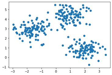
Which of the following would be closest to the command print (kmeans. cluster_centers_)?

• [ 1.0 4.0 2.0 1.0 -1.5 3.0]
• [[ 1.0 4.0]

[ 2.0 1.0]

[-1.5 3.0]]

• [[ 1.0 2.0 -1.5]

[ 4.0 1.0 3.0]]

Question 26: How does creating a regression model differ from solving a classification problem?

• Classification labels are discrete, regression output is continuous
• Classification models are unsupervised, regression models are supervised
• Classification techniques require vector data, regression techniques require scalar data

Question 27: Given this data set:

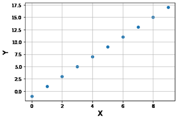
after this code runs:

from sklearn import linear_model
model = linear_model. LinearRegression ()
model.fit (X, Y)
print (model. score (X, Y))

Which of the following choices would best approximate the screen output?

• 0.0
• 1.0
• 10.0

Question 28: Assume the LinearRegression method from scikit-learn with its default parameters has been used to fit a model. In order for the OLS method in statsmodels to yield an equivalent model for the same training set, what method must be applied before creating the model?

• add_constant
• add_lag
• add_mean

Question 29: An autoregressive integrated moving average (ARIMA) model attempts to remove non-stationary components of a time series by doing which of the following?

• Adding values to their previous values
• Multiplying values by their previous values
• Subtracting values from their previous values

Question 30: What screen output will result after the following instructions execute?

a = [‘height’, ‘width’, ‘stop’, ‘going’]
print(a [2][3]) 

• i
• p
• stop

going

Question 31: Assuming the random module has been imported, which of the following instructions will generate a random floating-point number between 0 and 1?

• random. random (0,1)
• random. random (1)
• random. random ()

Question 32: Which of the following instructions will plot the function f(x)=x� (�) =� over the interval [1,4]?

• import matplotlib. pyplot as plt

plt. plot ([1,2,3,4], [1,1,1,1])

• import matplotlib. pyplot as plt

plt. plot ([1,2,3,4], [1,2,3,4])

• import matplotlib. pyplot as plt

plt. plot ([1,1], [2,2], [3,3], [4,4])

Question 33: Given the instructions

import numpy as np
B = np. array ([[-3,1], [3, –1], [4,5], [7,8]])

Which of the following instructions will result in the output [1 3 5 8]?

• print (B.max ())
• print (B.max(axis=0))
• print (B.max(axis=1))

Question 34: In addition to saving data, the savetxt method also allows you to do what?

• Delete an existing file
• Change the data type
• Add a header to the data

Question 35: To randomly sample a dataset without replacement, which of the following numpy random methods can be used with the input replace=False?

• shuffle
• choice
• randint

Question 36: Given a dataset array named data, consider the following calculation:

x = scipy. stats. zscore(data)

What conclusion can be drawn if a value in the array x is equal to zero?

• Its corresponding data value should be discarded.
• Its corresponding data value has 0% confidence interval.
• Its corresponding data value is equal to the mean.

Question 37: If you need to perform indexing in pandas in a manner similar to indexing a numpy array, which of the following methods should you use?

• iloc
• insert
• items

Question 38: Consider this set of instructions:

import numpy as np
import pandas as pd
b = np. random. randint (5,10, size= (5, 7))
a = pd. DataFrame(b)

Which of the following instructions will output rows with indices 2 through 4?

• print (a [2:5])
• print (a [2:5:])
• print (a [:] [2:4])

Question 39: The read_csv method should be used for which type of data files?

• Text files whose row data is separated by commas
• SQL files whose data stored in a relational database
• Binary data files in which row data is stored sequentially

Question 40: Given a dataframe df, if the instruction df. plot. hist(bins=10) will superimpose histograms from each column on a single plot, which instruction will create separate histogram plots for each column?

• df. diff. hist(bins=10)
• df. diff (). hist (bins=10)
• df. hist(bins=10). diff ()

Question 41: Assume you are given data in the form of frequency/counts and wish to analyze the data using histogram techniques. Which of the following would be the most appropriate method for doing so?

• catplot
• distplot
• relplot

Question 42: Which of the following best describes the case where a supervised learning algorithm is able to memorize training examples without being able to generalize well?

• Overfitting
• Oversampling
• Overtraining

Question 43: Given a supervised training set consisting of a feature matrix X and a target matrix y, consider this code:

import numpy as np
from sklearn import tree
from sklearn.model_selection import train_test_split
 
X_train, X_test, y_train, y_test = train_test_split(X, y)
test_scores = [ ]
dvals = np.arange(1, 10)
for i in dvals:
  dtree = tree.DecisionTreeClassifier(max_depth = i).fit(X_train, y_train)
  test_scores.append(dtree.score(X_test,y_test))

Which of the following instructions will find the optimal tree depth based on the list of test scores?

• dvals[np.max(test_scores)]
• dvals [np. argmax(test_scores)]
• dvals [np. fsolve(test_scores)]

Question 44: After applying a clustering algorithm from sklearn. cluster, how can the cluster membership of each vector in the training set be determined?

• By referencing the labels_ attribute
• By creating a scatter plot of the training data
• By computing the inverse of the clustering algorithm

Question 45: Which of the following clustering algorithms exclusively applies centroids in order to compute cluster membership?

• Only K-means clustering
• Only agglomerative clustering
• Both K-means and agglomerative clustering

Question 46: Which of the following is true regarding simple linear regression?

• The sum of the residuals is minimized
• The sum of the square of the residuals is minimized
• The sum of the absolute value of the residuals is minimized

Question 47: Assume this linear regression:

from sklearn import linear_model
model = linear_model. LinearRegression ()
model.fit (X, Y)

has been performed on this dataset:

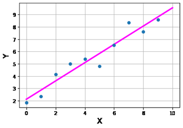
Which of the following sets of commands are needed in order to construct the magenta regression line shown in this figure?

• xt = np. linspace (0.0, 10.0, 100)

yt = model. predict(xt)

• xt = np. linspace (0.0, 10.0, 100)

xt = xt [:np. newaxis]

yt = model. predict(xt)

• xt = np. linspace (0.0, 10.0, 100)

xt = xt [:np. newaxis]

s = model. predict (xt, yt)

Question 48: Which of the following approaches can be applied in order to guard against overfitting?

• Analyze the residuals
• Perform cross-validation
• Minimize mean squared error

Question 49: Assuming this import has been invoked:

import statsmodels.graphics.tsaplots as sgt

What is the command for generating a plot of the partial autocorrelation function on a time series tsdata with a lag of 10 data points?

• sgt.pacf(tsdata, lags = 10)
• sgt.plot.pacf(tsdata, lags = 10)
• sgt.plot_pacf(tsdata, lags = 10)

Question 50: In data science, which of the following best characterizes how a model is used?

• To represent a system
• To begin a data science pipeline
• To determine patterns within data

Question 51: By default, where are your Google Colab notebooks stored?

• On your local drive
• On your thumb drive
• On your Google drive

Question 52: What Python keyword must be used when creating a function?

• func
• def
• init

Question 53: In the random module, what method can be used to set the initial value of the random number generator?

• init
• rand
• seed

Question 54: Which of the following instructions will create this matrix?

A=[012345]

• import numpy as np

A = np. array ([[0,1], [2,3], [4,5]])

• import numpy as np

A = np. array ([[0,2,4], [1,3,5]])

• import numpy as np

A = np. array (2,3, [0,2,4,1,3,5])

Question 55: Which of the following methods can be used to load and store data in plain text format?

• loadtxt and savetxt
• loadtext and savetext
• loadplntxt and saveplntxt

Question 56: Which of the following methods can be used to set the seed of a random number generator using the numpy module?

• RandomInit
• RandomSet
• RandomState

Question 57: Given this set of instructions:

from scipy import stats

u = stats. uniform (90, 100)

u.rvs (1000). mean ()

The computed mean would be closest to which of the following values?

• 45
• 95
• 140

Question 58: Which pandas method can be used to generate a report providing the number of non-null entries in each column of a dataframe?

• iloc
• info
• items

Question 59: Given this set of instructions:

import pandas as pd

A = pd. DataFrame (np. random. randn (5,5))

c = pd. Series ([1,2,3,4,5])

What is the effect of the operation A+c?

• Add each element of c to each row of A
• Add each element of c to each column of A
• Concatenate the series c as a new column in A

Question 60: Which of the following instructions will read an Excel spreadsheet into a dataframe df?

• import pandas as pd

df = pd. read_excel(read_file_name)

• import pandas as pd

df = DataFRame ()

df. read_excel(read_file_name)

• import pandas as pd

pd. read_excel (df, read_file_name)

Question 61: The default plotting mode for the Seaborn relplot command is equivalent to which of the following commands?

• histplot
• lineplot
• scatterplot

Question 62: Consider this barplot from a dataframe containing three columns: “day”, “total bill”, and “smoker”:

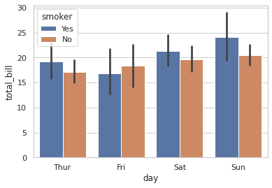
What is the name of the input parameter that enables the nesting of the “smoker” column along the “day” axis?

• hue
• level
• orient

Question 63: Which of the following is a parameter that can be modified when using the Decision Tree Classifier method?

• feat_weight
• min_depth
• random_state

Question 64: Distance-based clustering algorithms ideally generate clusters having which of the following properties?

• Small intra-cluster distances, large inter-cluster distances
• Large intra-cluster distances, small inter-cluster distances
• Large intra-cluster distances, large inter-cluster distances

Question 65: In simple linear regression with a single independent variable, which of the following is true?

• A positive correlation coefficient implies a positive slope
• A positive correlation coefficient implies a negative slope
• A negative correlation coefficient implies a positive slope

Question 66: After these instructions execute:

from sklearn. linear_model import LinearRegression

import numpy as np

X = np. array ([i for i in range (10)])

Y = np. array ([i for i in range (20,40,2)])

X = X [:np. newaxis]

Y = Y [:np. newaxis]

model = LinearRegression ()

model.fit (X, Y)

print (model. coef_, model. intercept_)

Which of the following choices would best approximate the screen output?

• [[1.]] [20.]
• [[2.]] [10.]
• [[2.]] [20.]

Question 67: When is underfitting most likely to occur?

• When a model perfectly learns the training set
• When a model is inflexible to new observations
• When the training data is too complex for the model

Question 68: When considering an AR(p) autoregressive time series model of order p, what does the parameter p refer to?

• The power that the time series values are raised to
• The pth statistical moment of the time series distribution
• The number of previous times used to predict the present time

Question 69: Which of the following is the correct syntax for importing the ARIMA method from stats models?

• from statsmodels.tsa. model import ARIMA
• from statsmodels.tsa. arima_model import ARIMA
• from statsmodels.tsa. arima. model import ARIMA

Question 70: Assuming this linear regression:

import numpy as np

from sklearn. linear_model import LinearRegression

from sklearn. metrics import r2_score

model = LinearRegression (). fit (X, Y)

is performed on this data set:

Which of the following best approximates the output from the instruction print (r2_score (Y, model. predict(X)))?

• 0.0
• 0.5
• 1.0

Question 71: Given the Seaborn ‘mpg’ dataset in CSV format, you will write a function named my_data_query that loads the dataset into a Pandas dataframe.  Your function will then select and sort values from the mpg column based on conditions that you set for the cylinders, weight, and horsepower columns.

Function call syntax:  z = my_data_query (dataset_name, condition_list), where:

dataset_name = ‘mpg.csv’

condition_list = input list of condition values (see example below) for the cylinders, weight and horsepower columns

z = sorted numpy vector of unique values from the mpg column

The condition_list will consist of four elements:

condition_list [0] = [‘cylinders’, nyclinders] where nyclinders = the number of cylinders used to extract values equal to nyclinders.

condition_list [1] = [‘weight’, weight] where weight = car weight used to extract values less than weight.

condition_list [2] = [‘horsepower’, horsepower] where horsepower = car horsepower used to extract the horsepower largest values.

condition_list [3] = [‘mpg’] refers to the mpg column

Within your function, you are to use the condition_list as follows:

Select all rows from the dataframe where the condition (‘cylinders’ == nyclinders) and (‘weight’ < weight) is satisfied.

From this selection, you will then select rows containing the largest values in the ‘horsepower’ column.

From this selection, you will extract the unique values from the ‘mpg’ column, sort them from lowest to highest, and return them as a numpy vector.

Example usage:

dataset_name = ‘mpg.csv’

condition_list = [[‘cylinders’, 8], [‘weight’, 4000],

                  [‘horsepower’, 30], ‘mpg’]

z = my_data_query (dataset_name, condition_list)

should return the values

array ([11., 13., 14., 15., 16., 16.5, 17., 17.5, 18.,

       18.1, 18.2, 18.5, 19.2, 19.4, 20.2]

Note: The file path for the CSV file location is already set for you in the answer preload.

Answer:(penalty regime: 10, 20, … %)

def my_data_query (dataset_name, condition_list):

  dataset_path = ‘/var/lib/seaborn-data/’

  dataset_filename = dataset_path + dataset_name 

  df = pd. read_csv(dataset_filename)

    cylinders_condition = condition_list [0]

    weight_condition = condition_list [1]

    horsepower_condition = condition_list [2]

    filtered_df = df [(df [cylinders_condition [0]] == cylinders_condition [1]) &

                     (df [weight_condition [0]] < weight_condition [1])]

    sorted_df = filtered_df. nlargest (1, horsepower_condition [0])

    sorted_mpg_values = np. sort (sorted_df [condition_list [3]]. unique ())

    return sorted_mpg_values

Question 72: Write a function named my_cluster_comparison that will cluster an input training matrix using both K-means clustering and agglomerative clustering. To compare the cluster members for each technique, it is unlikely that the computed cluster labels will end up being the same. To resolve this issue, your function will map the agglomerative clustering labels to the K-means clustering labels as follows (assuming the same number of clusters for each technique): After using the input data to fit both an AgglomerativeClustering model and a KMeans model, for each agglomerative cluster.

Compute the centroid of the agglomerative cluster (such as by using the numpy mean method).

Using the centroids obtained by fitting the KMeans model to the input training set, apply the neighbors method to fit a nearest neighbor model using one neighbor.

Use the predict method from your nearest neighbor object to classify the agglomerative centroid computed in step 1. This step will correctly associate the agglomerative cluster with the appropriate KMeans label.

Update the input training vectors with the new agglomerative label.

Return the training vector indices where the new agglomerative indices differ from the Kmeans indices.

Function call syntax results = my_cluster_comparison (X_train, nc, random_state_val)  

X_train = input p×n

 numpy matrix containing p

 samples and n

 features.

nc = integer describing the number of clusters

random_state_val= integer for setting the random state

You may assume

import numpy as np

from sklearn. cluster import KMeans

from sklearn. cluster import AgglomerativeClustering

from sklearn import neighbors

from sklearn. model_selection import train_test_split

have been invoked.

Example test case:

random_state_val = 50

np. random. seed(seed=random_state_val)

npts = 25

dim = 2

a=1

c0_mu = np. array ([a, a])

c0_data = c0_mu + np. random. normal (0, 1, size= (npts, dim))

c1_mu = np. array ([-a, a])

c1_data = c1_mu + np. random. normal (0, 1, size= (npts, dim))

c2_mu = np. array ([a, -a])

c2_data = c2_mu + np. random. normal (0, 1, size= (npts, dim))

c3_mu = np. array ([-a, -a])

c3_data = c3_mu + np. random. normal (0, 1, size= (npts, dim))

X = np. concatenate ((c0_data, c1_data, c2_data, c3_data), axis=0)

nc = 4

X_train, X_test = train_test_split (X, test_size=0.20, random_state=random_state_val)

results = my_cluster_comparison (X_train, nc, random_state_val)

should return a value of

(array ([ 1, 2, 9, 12, 13, 14, 28, 29, 34, 42, 47, 57, 59, 60, 66, 67, 74]),)

for results.

Notes: Try to keep the computed labels as type integer

Answer:(penalty regime: 0 %)

def my_cluster_comparison (X_train, nc, random_state_val):

  kmns = KMeans (n_clusters=nc, random_state=random_state_val). fit(X_train)

  aggm = AgglomerativeClustering(n_clusters=nc). fit(X_train)

  n_neighbors = 1

  knn = neighbors. KNeighborsClassifier(n_neighbors)

  aggm_list = [ ] # extra storage if needed

  new_aggm_labels = np. zeros ((aggm. labels_. shape), dtype = np.int32)

  for label in range(nc):

        cluster_points = X_train [aggm. labels_ == label]

        centroid = np. mean (cluster_points, axis=0)

        knn.fit (kmns. cluster_centers_, kmns. labels_)

        nearest_neighbor_label = knn. predict([centroid])

        new_aggm_labels [aggm. labels_ == label] = nearest_neighbor_label 

  return np. where (new_aggm_labels! = kmns. labels_)

Question 73: Write a function name eval_normal_pdf that, given an input mean and standard deviation, will evaluate the probability density function (PDF) for a normal distribution at a specific set of input points using two different methods:

Explicit calculation using numpy: f(x)=12π√σe−12(x−μ)2σ2     

Using the norm.pdf method in scipy. stats 

Function syntax:  eval_normal_pdf (x, mu, sigma)

Function inputs:

x is a number vector of points at which to evaluate the PDF

mu is the mean

sigma is the standard deviation

Function output:  return y1, y2

y1 is the PDF using method 1

y2 is the PDF using method 2

You may assume

from scipy. stats import norm

import numpy as np

from math import sqrt, pi

have been invoked.

Example:

x = np. array ([-3, -2, -1, 0, 1, 2, 3])

mu = -1

sigma = 2

f1, f2 = eval_normal_pdf (x, mu, sigma)

would return PDFs evaluated at points defined by the vector x.

Answer:(penalty regime: 10, 20, … %)

def eval_normal_pdf (x, mu, sigma):

    y1 = 1 / (sqrt (2 * pi) * sigma) * np.exp (-0.5 * ((x – mu) / sigma) **2)

    y2 = norm.pdf (x, mu, sigma)   

    return y1, y2

Question 74: Which of the following would be considered a part of the data exploration process?

• Cleansing the data
• Creating a data plot
• Validating a data model

Question 75: Cluster sampling and simple random sampling are both examples of what kind of sampling?

• Data sampling
• Stratified sampling
• Probability sampling

Question 76: Which of the following commands will allow you to install a module into a Google Colab environment?

• ! Pip installs
• #Pip installs
• @Pip installs

Question 77: Which of the following instructions will create this matrix?

A= [0 0.1 0.2 0.3 0.4 0.5 0.6 0.7 0.8 0.9 1.0]

• import numpy as np

A = np. linspace (0,0.1,1)

• import numpy as np

A=np.linspace(0, 1, 10)

• import numpy as np

A = np. linspace (0,0.1,1)

Question 78: Given the instructions

import numpy as np

A = np. array ([[0,4,8,12,16], [1,5,9,13,17], [2,6,10,14,18], [3,7,11,15,19]])

which of the following instructions is equivalent to print (A [-2:])?

• print (A [0:])
• print (A [2:])
• print (A [3:])

Question 79: Given this instruction for dataframe df:

df. plot. scatter (x=’c’, y=’d’, color=’red’, marker=’x’, s=10)

What is the purpose of the parameter s?

• It sets the size of the marker
• It specifies number of points to plot
• It sets number of tickmarks for the axes

Question 80: In addition to plotting quartile ranges, the boxplot method also computes and superimposes which of the following?

• Outlier points
• Kernel estimate
• Confidence interval

Question 81: After applying the train_test_split method, which of the following methods would be most appropriate to apply to the test set?

• fit
• predict
• make_classification

Question 82: Given a feature matrix X and assuming this instruction has executed:

from sklearn import preprocessing

Which of the following instructions will scale each feature so that they have zero mean and unit variance?

• scaler = preprocessing. StandardScaler (). fit(X)

X_scaled = scaler. transform(X)

• scaler = preprocessing. Normalizer (). fit(X)

X_scaled = scaler. transform(X)

• scaler = preprocessing. QuantileTransformer (). fit(X)

X_scaled = scaler. transform(X)

Question 83: What is the default mode for the init parameter in a sklearn. cluster. KMeans object?

• ‘batch’
• ‘k-means++’
• ‘random’

Question 84: Which of the following statements is true?

• K-means clustering requires the number of clusters as an input parameter
• Agglomerative clustering requires the number of clusters as an input parameter
• Both agglomerative and K-means clustering require the number of clusters as an input parameter

Question 85: Assume statsmodels has been used to fit an ordinary least squares model of the form y=β1×1+β2×2+c and output an object named model. Which of the following instructions will reference the constant term in the model after running the command results = model.fit ()?

• results. params [0]
• results. params [1]
• results. params [2]

Question 86: In data science, what would text, numbers, images, audio, and video be different examples of?

• Data types
• Feature types
• Variable types

Question 87: What will be the result after these commands execute?

import numpy

A = np. array ([[0,4,8,12,16], [10,20,30,40,40],[100,200,300,400,400]])

print(np.sum(A[A<5]))

• 0
• 2
• 4

Question 88: Assuming import numpy as np has been invoked, what will the np. save method do?

• Save a single array to a single file in. npy format
• Save several arrays into a single file in compressed. npy format
• Save several arrays into a single file in uncompressed. npz format

Question 89: When using the histplot command, what is the effect of setting the kde input parameter to a value of True?

• A cdf estimate is plotted
• A pdf estimate is superimposed
• The default bin width can be modified

Question 90: Which of the following commands would create a bar plot of medians with a confidence interval of 90 percent?

• from numpy import median

import seaborn as sns

sns. barplot (x=’day’, y=’tip’, data=tips, estimator=’median’, ci = 90)

• from numpy import median

import seaborn as sns

sns. barplot (x=’day’, y=’tip’, data=tips, estimator=median, ci = 0.90)

• from numpy import median

import seaborn as sns

sns. barplot (x=’day’, y=’tip’, data=tips, estimator=median, ci = 90)

Question 91: Which of the following is true regarding any data set used to train a supervised learning model?

• Input values are processed as scalar quantities
• Input values are produced using nonrandom data
• Input values are paired with desired output targets

Question 92: Consider instantiating a sklearn. cluster. Agglomerative object. If the distance_threshold parameter is being set to a specific value (i.e., not equal to None) in order to validate a given cluster model, how should the following parameters be set?

• n_clusters must be set to None and compute_full_tree must be set to True
• n_clusters must be set to a value of -1 and compute_full_tree must be set to False
• n_clusters must be set to an integer greater than one and compute_full_tree must be set to True

Question 93: Using the scientific method in data science applications, one option is to apply inductive reasoning. What other type of reasoning is common in data science?

• Deductive reasoning
• Reductive reasoning
• Subtractive reasoning

Question 94: In the process of data sampling, when attempting to identify the true parameters of a population, why is it sensible to consider statistical bias?

• Because the population sample size must be verified
• Because the deviation of the estimate must be characterized
• Because the resulting parameters could be skewed toward the true parameters

Question 95: Given raw data values from a population, assume that:

            X

 = a raw data values

             μ

 = population means

             σ

 = population standard deviation

What scipy. stats method can be used to calculate the equation (X−μ)/σ?

• kurtosis
• skew
• zscore

Question 96: Which of the following methods can be used to replace any missing values in a dataframe with a specified replacement value?

• assign
• fillna
• insert

Question 97: When using the histplot command, what is the effect of setting the kde input parameter to a value of True?

• A cdf estimate is plotted
• A pdf estimate is superimposed
• The default bin width can be modified

Question 98: When computing and plotting linear regressions with either lmplot or regplot, in addition to both methods accepting pandas dataframes as valid input data, which of the following is true?

• Only lmplot accepts numpy arrays as input
• Only regplot accepts numpy arrays as input
• Both lmplot and regplot accept numpy arrays as input

Question 99: Given a feature matrix X and assuming this instruction has executed:

from sklearn. decomposition import PCA

Which of the following instructions will attempt to determine the optimal number of components in the dimensionally reduced set of feature vectors?

• pca = PCA (n_components = None)

pca.fit(X)

• pca = PCA (n_components = ‘svd’)

pca.fit(X)

• pca = PCA (n_components = ‘mle’)

pca.fit(X)

Question 100: Which of the following data mining problems would be most appropriate to solve using an unsupervised learning algorithm?

• Recognizing images of license plates
• Classifying objects within images of natural scenery
• Classifying images of apples versus images of oranges

Question 101: Consider this snippet of code:

data = [ ]

for i in range (1, 11):

    kmeans = KMeans (n_clusters=i, init=’k-means++’, max_iter=300,

                    n_init=10, random_state=0)

    kmeans.fit(X)

What instruction should be inserted after the kmeans.fit(X) command that will build the list data and can be used to analyze the tradeoff between the inter-cluster sum of squared distances and the number of clusters?

• data. append (kmeans. mse_)
• data. append (kmeans. delta_)
• data. append (kmeans. inertia_)

Question 102: Assuming this multiple linear regression executes:

import numpy as np

from sklearn. linear_model import LinearRegression

X = np. array ([[1, 1], [1, 4], [2, 3], [3, 5]])

y = np.dot (X, np. array ([2, 4])) + 3

model = LinearRegression (). fit (X, y)

What type of numpy element is the quantity model. coef_?

• A numpy array
• A numpy scalar
• A numpy vector

Question 103: Assuming the ARIMA method has been imported and run on a data frame df with column name prices, how many moving averages model coefficients will this instruction generate?

model_ar2 = ARIMA (df. prices, order = (4,1,2))

• 1
• 2
• 4

Question 104: The mean squared error is an example of which of the following?

• A loss functions
• A hypothesis tests
• A sampling functions

Question 105: What is the effect of the following commands?

import matplotlib. pyplot as plt

plt. subplot (2, 1, 2)

• Referring to the right plot of two plots that are placed from left to right
• Referring to the top right corner plot of four plots placed within a square
• Referring to the bottom plot of two plots that are stacked on top of one another

Question 106: Given the instructions

import numpy as np

A = np. array ([[0,4,8,12,16], [1,5,9,13,17], [2,6,10,14,18], [3,7,11,15,19]])

which of the following instructions will yield the output 19?

• print (A [-1, -1])
• print (A [-1,3])
• print (A [3, -1])

Question 107: Which matplotlib method is most appropriate for plotting a probability mass function?

• hist
• quiver
• stem

Question 108: How does a dataframe differ from a numpy array?

• A dataframe is limited to two dimensions
• A numpy array is limited to one dimension
• A numpy array can contain heterogeneous data

Question 109: Which instruction should be applied to a dataframe a in order to determine the number of non-null values in each column?

• a.notna().count()
• a.notna().len()
• a.notna().sum()

Question 110: What is the expected output after these instructions execute?

from sklearn.neighbors import KNeighborsClassifier

X = [[0], [1], [3], [4]]

y = [0, 0, 2, 2]

knn = KNeighborsClassifier(n_neighbors = 1)

knn.fit(X, y)

print(knn.predict([[1.7]]))

• 0
• 1
• 2

Question 111: If ‘single’ is chosen for the linkage parameter in a sklearn. cluster. AgglomerativeClustering object, what cluster set distance is being computed?

• The distance between the centroids from two different clusters
• The distance between the two closest points from two different clusters
• The distance between the two farthest points from two different clusters

Question 112: Assume statsmodels has been used to build a model from a training set and form the object model. Which of the following instructions will allow you to visualize the model performance after running the command results = model.fit ()?

• print (results. render ())
• print (results. report ())
• print (results. summary ())

Question 113: When referring to time series data models such as AR and MA, which of the following best describes the meaning of wide-sense stationary?

• The model coefficients are the same for each value of t
• The value of each sample Xt is the same for each value of t
• The mean of the distribution of each sample Xt is the same for each value of t